Reporting Multiple Regressions in APA format – Part One
So this is going to be a very different post from anything I have put up before. I am writing this because I have just spent the best part of two weeks trying to find the answer myself without much luck. Sure I came across the odd bit of advice here and there and was able to work a lot of it out, but so many of the websites on this topic leave out a bucket load of the information, making it difficult to know what they are actually going on about. So after two weeks of wading through websites, texts book and having multiple meetings with my university supervisors, I thought I would take the time to write up some instructions on how to report multiple regressions in APA format so that the next poor sap who has this issue doesn’t have to waste all the time I did. If you have no interest in statistics then I recommend you skip the rest of this post.
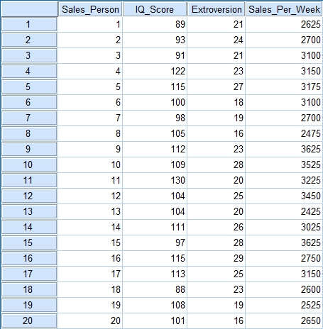
Ok let’s start with some data. Here is some that I pulled off the internet that will serve our purposes nicely. Here we have a list of sales people, along with their IQ level, their extroversion level and the total amount of money they made in sales this week. We want to see if IQ level and extroversion level can be used to predict the amount of money made in a week.
Now I am not going to show you how to enter the data into SPSS, if you don’t know how to do that I recommend you find out first and then come back. However, I will show you how to calculate the regression and all of the important assumptions that go along with it.
In SPSS you need to click Analyse > Regression > Linear and you will get this box, or one very much like it depending on your version of SPSS, come up.
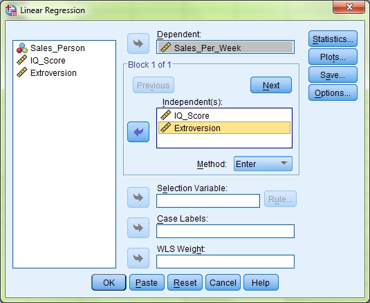
The first thing to do is move your Dependent Variable, in this case Sales Per Week, into the Dependent box. Next move the two Independent Variables, IQ Score and Extroversion, into the Independent(s) box. We are going to use the Enter method for this data, so leave the Method dropdown list on its default setting. We now need to make sure that we also test for the various assumptions of a multiple regression to make sure our data is suitable for this type of analysis. There are seven main assumptions when it comes to multiple regressions and we will go through each of them in turn, as well as how to write them up in your results section. These assumptions deal with outliers, collinearity of data, independent errors, random normal distribution of errors, homoscedasticity & linearity of data, and non-zero variances. But before we look at how to understand this information let’s first set SPSS up to report it.
Note: If your data fails any of these assumptions then you will need to investigate why and whether a multiple regression is really the best way to analyse it. Information on how to do this is beyond the scope of this post.
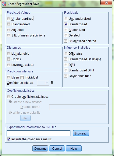
On the Linear Regression screen you will see a button labelled Save. Click this and then tick the Standardized check box under the Residuals heading. This will allow us to check for outliers. Click Continue and then click the Statistics button.
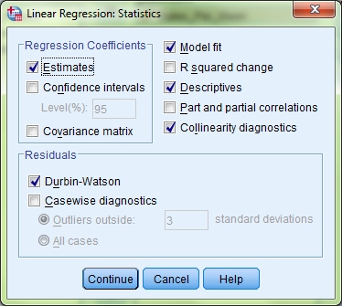
Tick the box marked Collinearity diagnostics. This, unsurprisingly, will give us information on whether the data meets the assumption of collinearity. Under the Residuals heading also tick the Durbin-Watson check box. This will allow us to check for independent errors. Click Continue and then click the Plots button.
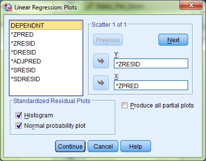
Move the option *ZPRED into the X axis box, and the option *ZRESID into the Y axis box. Then, under the Standardized Residual Plots heading, tick both the Histogram box and the Normal probability plot box. This will allow you to check for random normally distributed errors, homoscedasticity and linearity of data. Click Continue. As the assumption of non-zero variances is tested on a different screen, I will leave explaining how to carry that out until we get to it. For now, click OK to run the tests.
Outliers
The first thing we need to check for is outliers. If we have any they will need to be dealt with before we can analyse the rest of the results. Scroll through your results until you find the box headed Residual Statistics.
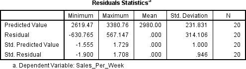
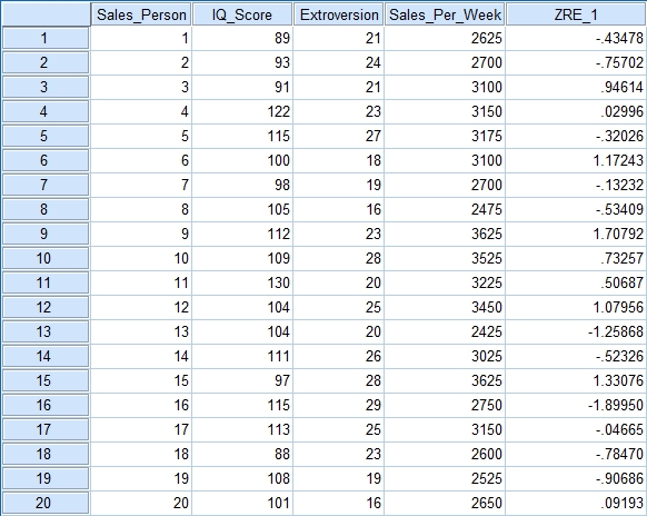
Look at the Minimum and Maximum values next to Std. Residual (Standardised Residual) subheading. If the minimum value is equal or below -3.29, or the maximum value is equal or above 3.29 then you have outliers. Now as you can see in this example data we don’t have any outliers, but if you do here is what you need to do. Go back to your main data screen and you will see that SPSS has added a new column of numbers titled ZRE_1. This contains the standardised residual values for each of your participants. Go down the list and if you find any values equal or over 3.29, or less than or equal to -3.29 then that participant is an outlier and needs to be removed.
Once you have done this you will need to analyse your data again, in the same way described above, to make sure you have fixed the issue. You may find that you have new outliers when you do this and these too will need to be dealt with. In my recent experiment I had to run the check for outliers six times before I got them all and the standardised residual values were under 3.29 & -3.29 respectively. When it comes to writing this up what you put depends on what results you got. But something along the lines of one of these sentences will do.
An analysis of standard residuals was carried out on the data to identify any outliers, which indicated that participants 8 and 16 needed to be removed.
An analysis of standard residuals was carried out, which showed that the data contained no outliers (Std. Residual Min = -1.90, Std. Residual Max = 1.70).
Collinearity
To see if the data meets the assumption of collinearity you need to locate the Coefficients table in your results. Here you will see the heading Collinearity Statistics, under which are two subheadings, Tolerance and VIF.
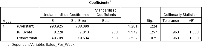
If the VIF value is greater than 10, or the Tolerance is less than 0.1, then you have concerns over multicollinearity. Otherwise, your data has met the assumption of collinearity and can be written up something like this:
Tests to see if the data met the assumption of collinearity indicated that multicollinearity was not a concern (IQ Scores, Tolerance = .96, VIF = 1.04; Extroversion, Tolerance = .96, VIF = 1.04).
Independent Errors
To check see if your residual terms are uncorrelated you need to locate the Model Summary table and the Durbin-Watson value.
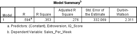
Durbin-Watson values can be anywhere between 0 and 4, however what you are looking for is a value as close to 2 as you can get in order to meet the assumption of independent errors. As a rule of thumb if the Durbin-Watson value is less than 1 or over 3 then it is counted as being significantly different from 2, and thus the assumption has not been met. Assuming it is you can write it up very simply like this:
The data met the assumption of independent errors (Durbin-Watson value = 2.31).
Random Normally Distributed Errors & Homoscedasticity & Linearity
I’m going to deal with these three things together as all the information comes from the same place. Now it is as this point that analysing the results becomes more of an art than a science as you need to look at some graphs and decide, pretty much for yourself, if they meet the various assumptions. We will start with the Histogram.
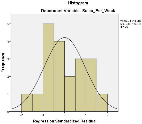
Now all going well this should have a nice looking normal distribution curve superimposed over a bar chart of your data. If you do then this means that your data has met the assumption of normally distributed residuals. However if you see something like the image below then you have problems.
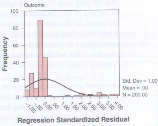
Copyright Andy Field – Discovering Statistics Using SPSS
Next you need to look at the Normal P-P Plot of Regression Standardized Residual, and yes I am aware that is says Observed Cum Prob on it and that this is highly amusing. That aside, this basically tells you the same thing as the Histogram, just in a different way.
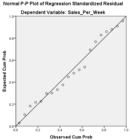
What you are looking for is for the dots to be on, or close, to the line running diagonally across the screen. If it looks something like the image below then again you have problems.
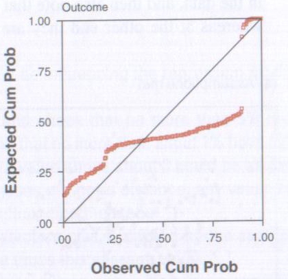
Copyright Andy Field – Discovering Statistics Using SPSS
When it comes to writing this information up you pretty much just have to describe what the two graphs look like. Something like this:
The histogram of standardised residuals indicated that the data contained approximately normally distributed errors, as did the normal P-P plot of standardised residuals, which showed points that were not completely on the line, but close.
Which brings us to the scatterplot, which will tell us if our data meets the assumptions of Homoscedasticity and Linearity. Now it is a bit hard to tell from the data we are using if these assumptions are met, as there are so few data points, and so I’m going to once again borrow some images from my textbook.
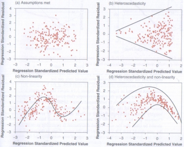
Copyright Andy Field – Discovering Statistics Using SPSS
Basically you want your scatterplot to look something like the top left hand image. If it looks like any of the others then one or both of the assumptions has not been met (The lines have been added to show the shape of the date, these will not appear on the actual scatterplot). Again this is more art than science and comes down to how you interpret the image. That said if your data has met all of the other assumptions then the chances are it will have met this one as well, so if you are a little unsure what the scatterplot is telling you, as you might be with the one produced with our data here, then look at your other results for guidance. And when it comes to writing it up, again you just say what you see.
The scatterplot of standardised predicted values (Note: You may want to call it the “scatterplot of standardised residuals” instead, either is good) showed that the data met the assumptions of homogeneity of variance and linearity.
Non-Zero Variances
As I said before I have left this one until last as you need to run a little bit of extra analysis to get the information you need. From the menus at the top select Analyse > Descriptive Statistics > Descriptives and you will get this box come up.

Add both your IVs and your DV to the Variable(s) box and then click Options.
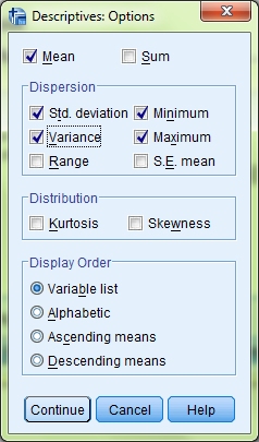
Check the Variance box under the heading Dispersion and then click Continue. Click OK to run the analysis and you will see this new table added to your results titled Descriptive Statistics.
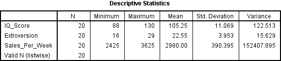
On this table you are looking for the heading Variance, and all you need to do is see whether the values are over zero or not. If they are then the assumption is met and can be reported like this:
The data also met the assumption of non-zero variances (IQ Scores, Variance = 122.51; Extroversion, Variance = 15.63; Sales Per Week, Variance = 152407.90).
Ok, so that is all the assumptions taken care of, now we can get to actually analysing our data to see if we have found anything significant.
To be continued in Part Two.
UPDATE 20/09/2013 – When writing this post I used a number of images that I took from a powerpoint presentation on regressions that I got from my University. While I had no idea where they originally came from it has been pointed out to me that they are from Andy Field’s book Discovering Statistics Using SPSS and as such I should have acknowledged this fact when making use of them. I am now doing so and apologise for this oversight, it was never my intention to imply that the images were of my own creation. Also let me recommend that you pick up a copy of Andy Field’s book. I have been meaning to do so for some time, but have been lacking the funds to do so, as I have heard nothing but good things about it from my fellow psychology students. I have been told it is a great resource for all your SPSS and statistical needs.
Leave a Reply